
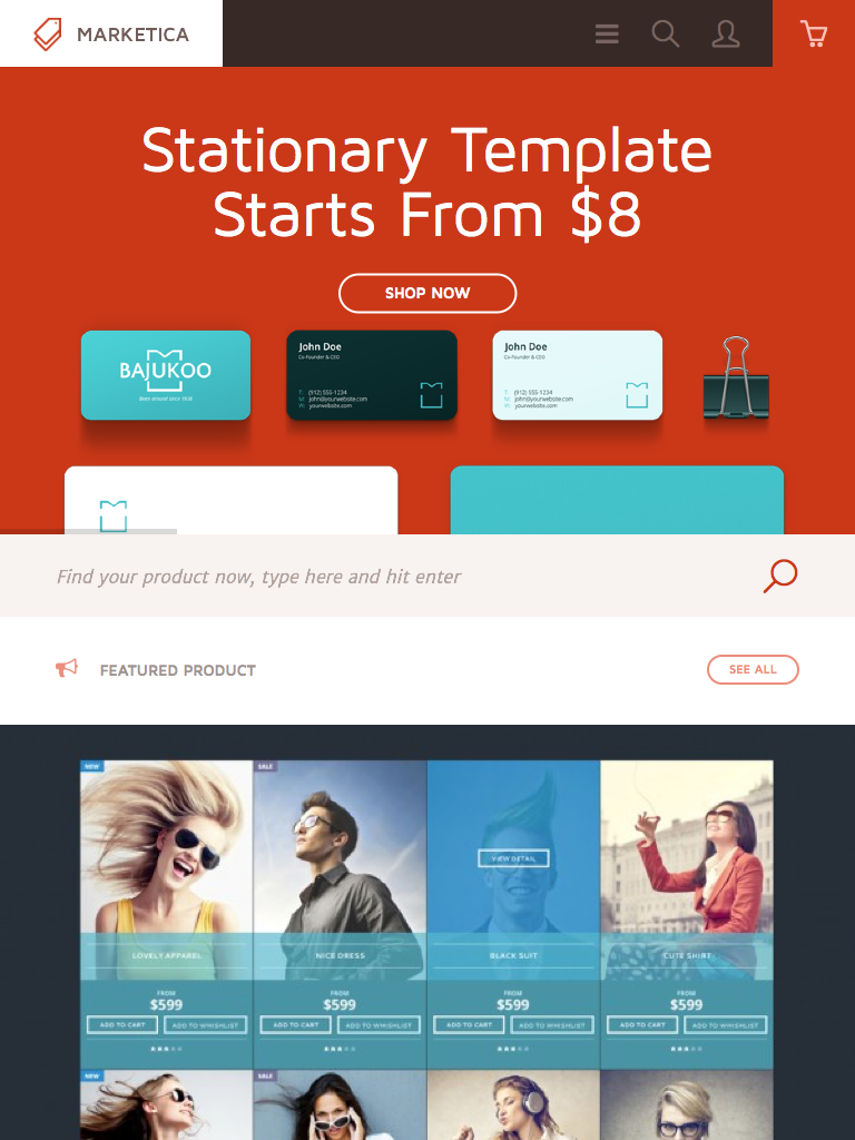
MARKETICA_PREVIEW/00-marketica-preview-sale37.jpg
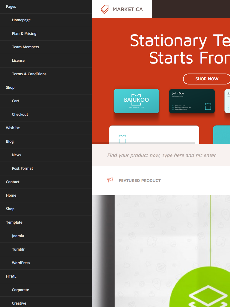
MARKETICA_PREVIEW/01_marketica2_homepage.png
MARKETICA_PREVIEW/02_marketica2_shop_page.png
MARKETICA_PREVIEW/03_marketica2_single_product_page.png
MARKETICA_PREVIEW/04_marketica2_cart_page.png
MARKETICA_PREVIEW/05_marketica2_checkout_page.png
MARKETICA_PREVIEW/06_marketica2_myaccount_login_page.png
MARKETICA_PREVIEW/07_marketica2_plan_and_pricing_page.png
MARKETICA_PREVIEW/08_marketica2_team_members_page.png
MARKETICA_PREVIEW/09_marketica2_contact_page_template.png
MARKETICA_PREVIEW/10_marketica2_blog_page.png
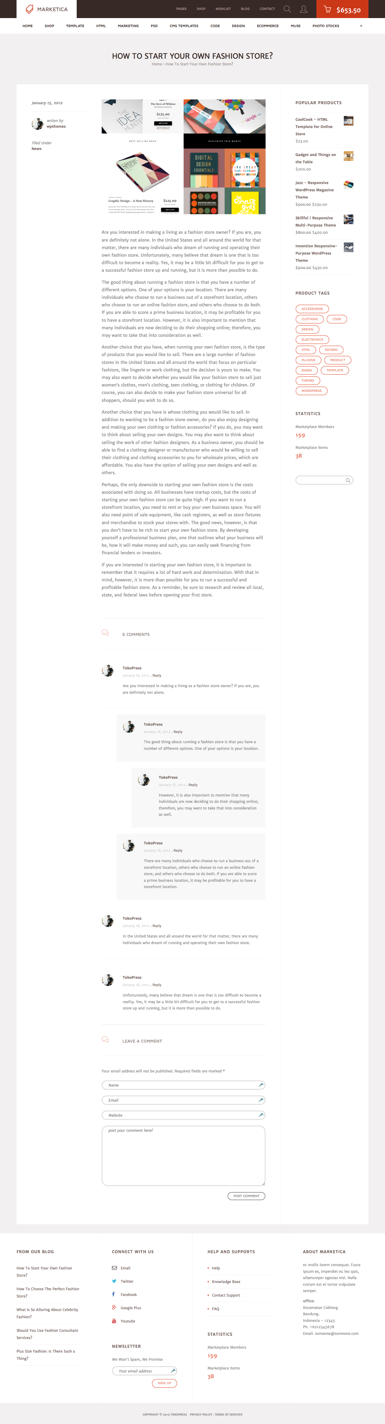
MARKETICA_PREVIEW/11_marketica2_blog_post_formats.png
MARKETICA_PREVIEW/12_marketica2_single_product_page.png
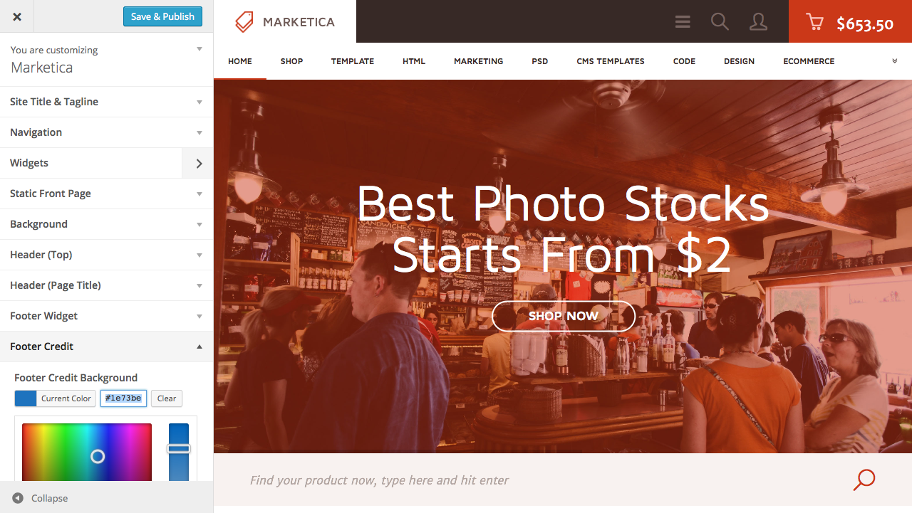
MARKETICA_PREVIEW/13_marketica2_theme_customizer.png
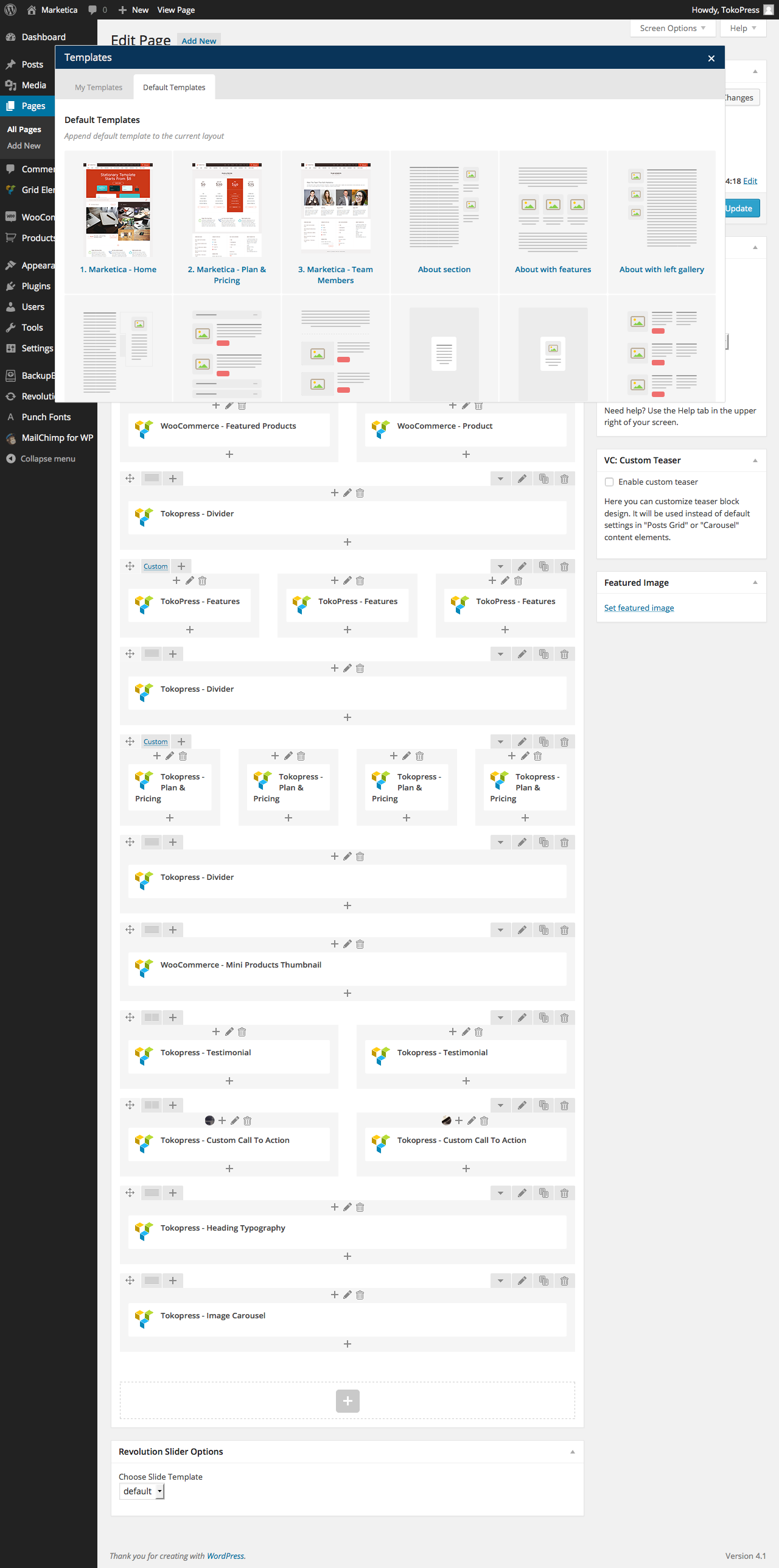
MARKETICA_PREVIEW/14_marketica2_visualcomposer_templates.png
MARKETICA_PREVIEW/15_marketica2_tablet_view.png
MARKETICA_PREVIEW/16_marketica2_tablet_view_offcanvas_menu.png
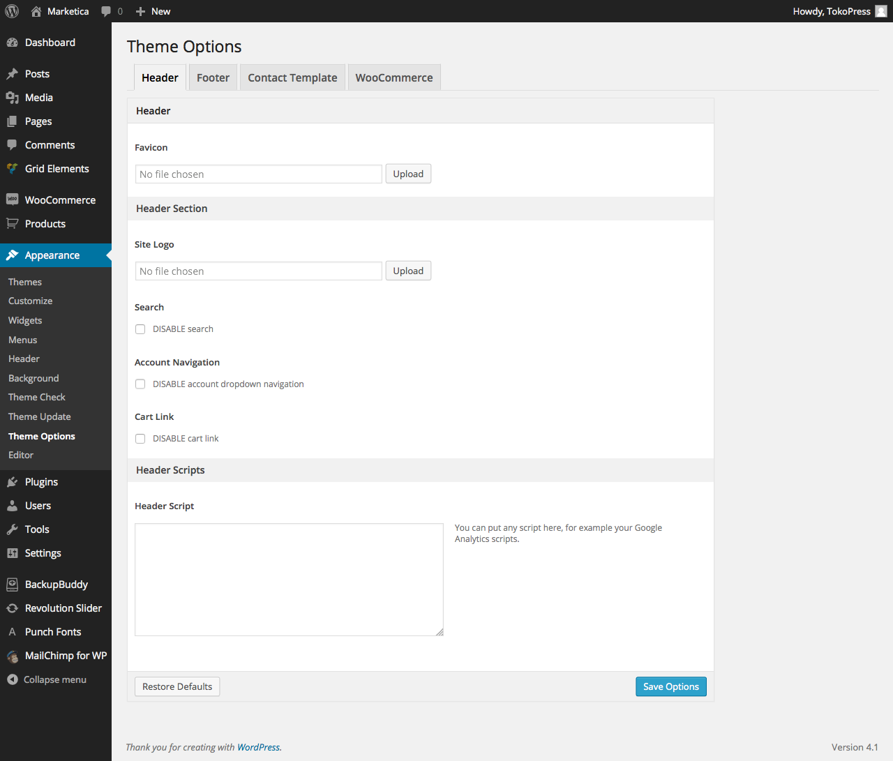
MARKETICA_PREVIEW/17_marketica2_themeoptions_header.png
MARKETICA_PREVIEW/18_marketica2_themeoptions_footer.png
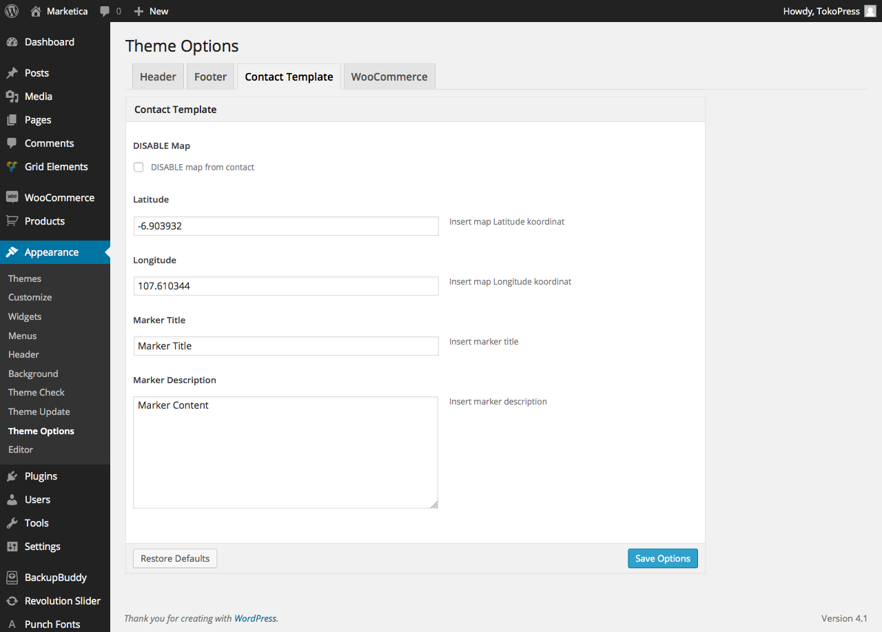
MARKETICA_PREVIEW/19_marketica2_themeoptions_contact.png
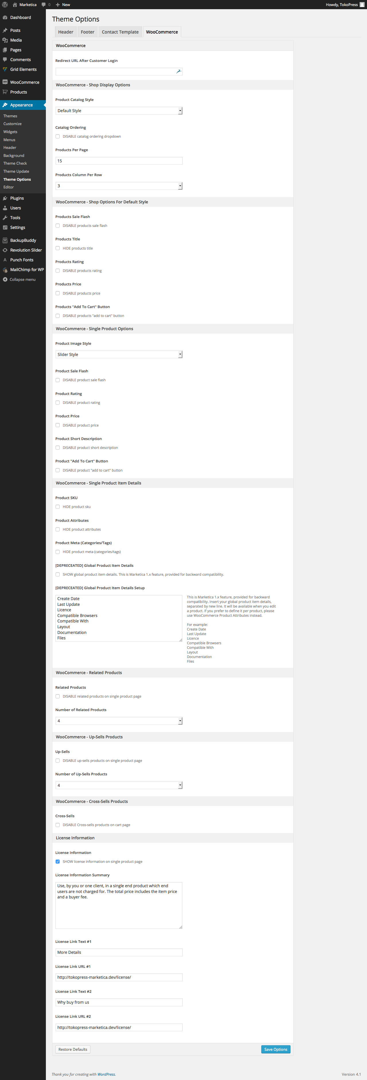
MARKETICA_PREVIEW/20_marketica2_themeoptions_woocommerce.png
MARKETICA_PREVIEW/21_marketica2_wcvendors_user_page.png
MARKETICA_PREVIEW/22_marketica2_wcvendors_vendor_page.png
MARKETICA_PREVIEW/23_marketica2_wcvendors_vendor_dashboard.png
MARKETICA_PREVIEW/24_marketica2_wcvendors_shop_settings.png
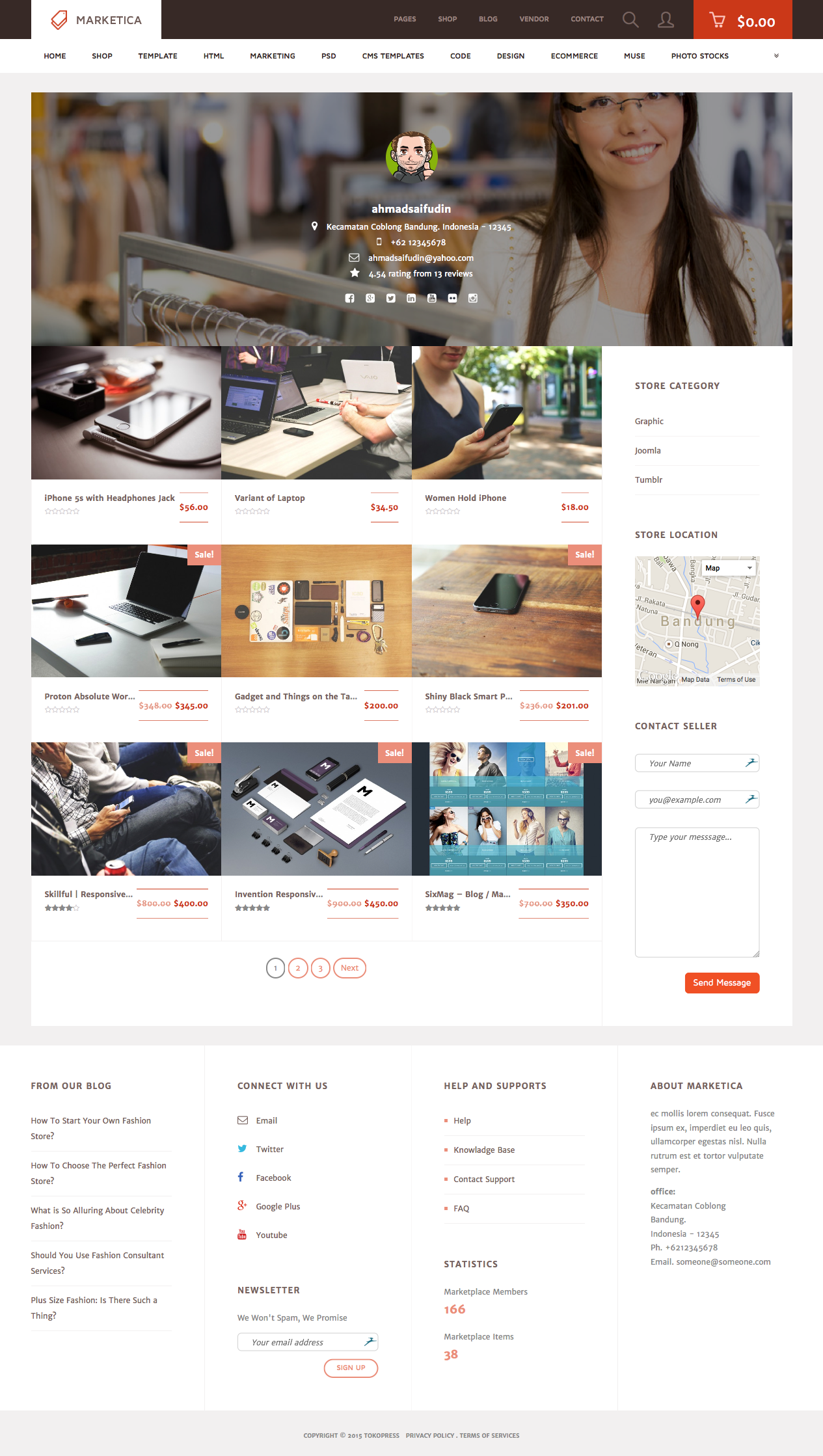
MARKETICA_PREVIEW/25_marketica2_dokan_vendor_store_page.png
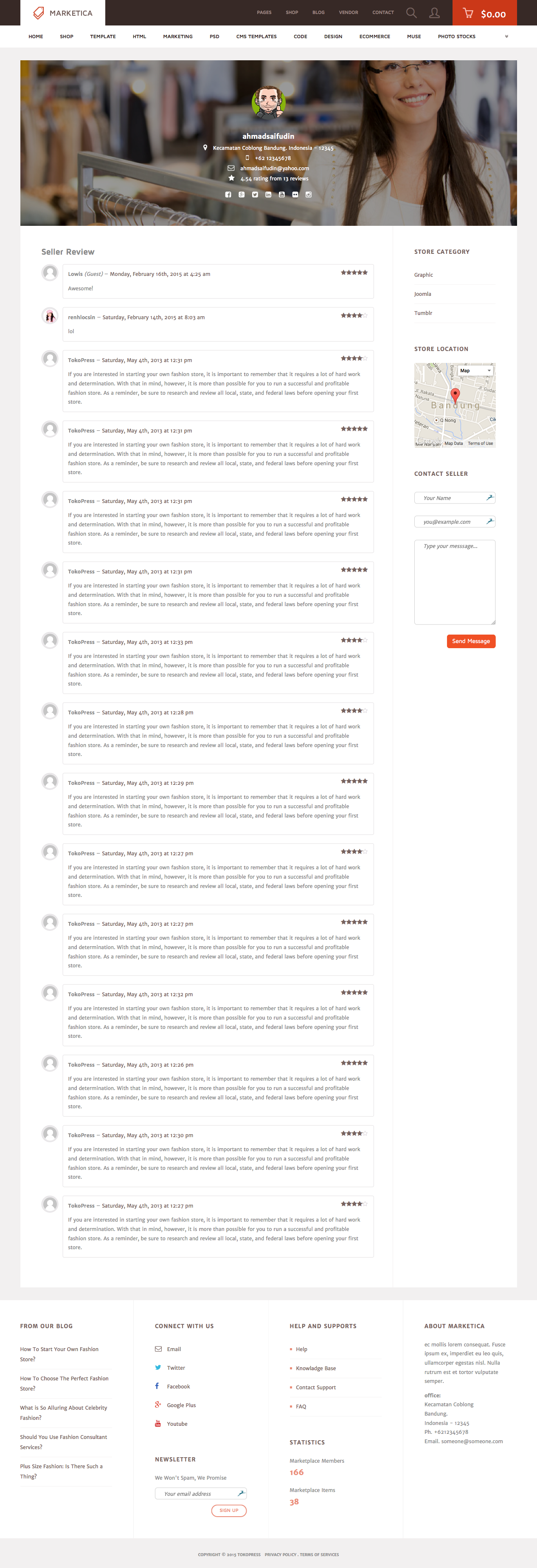
MARKETICA_PREVIEW/26_marketica2_dokan_vendor_review_page.png
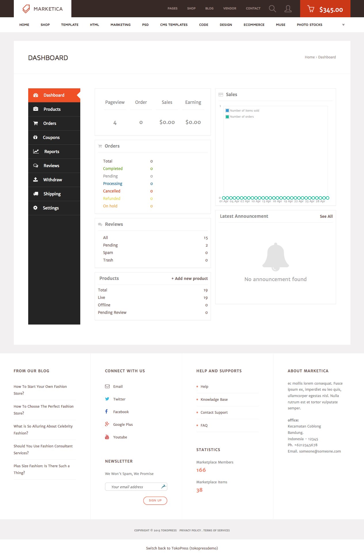
MARKETICA_PREVIEW/27_marketica2_dokan_vendor_dashboard_page.png
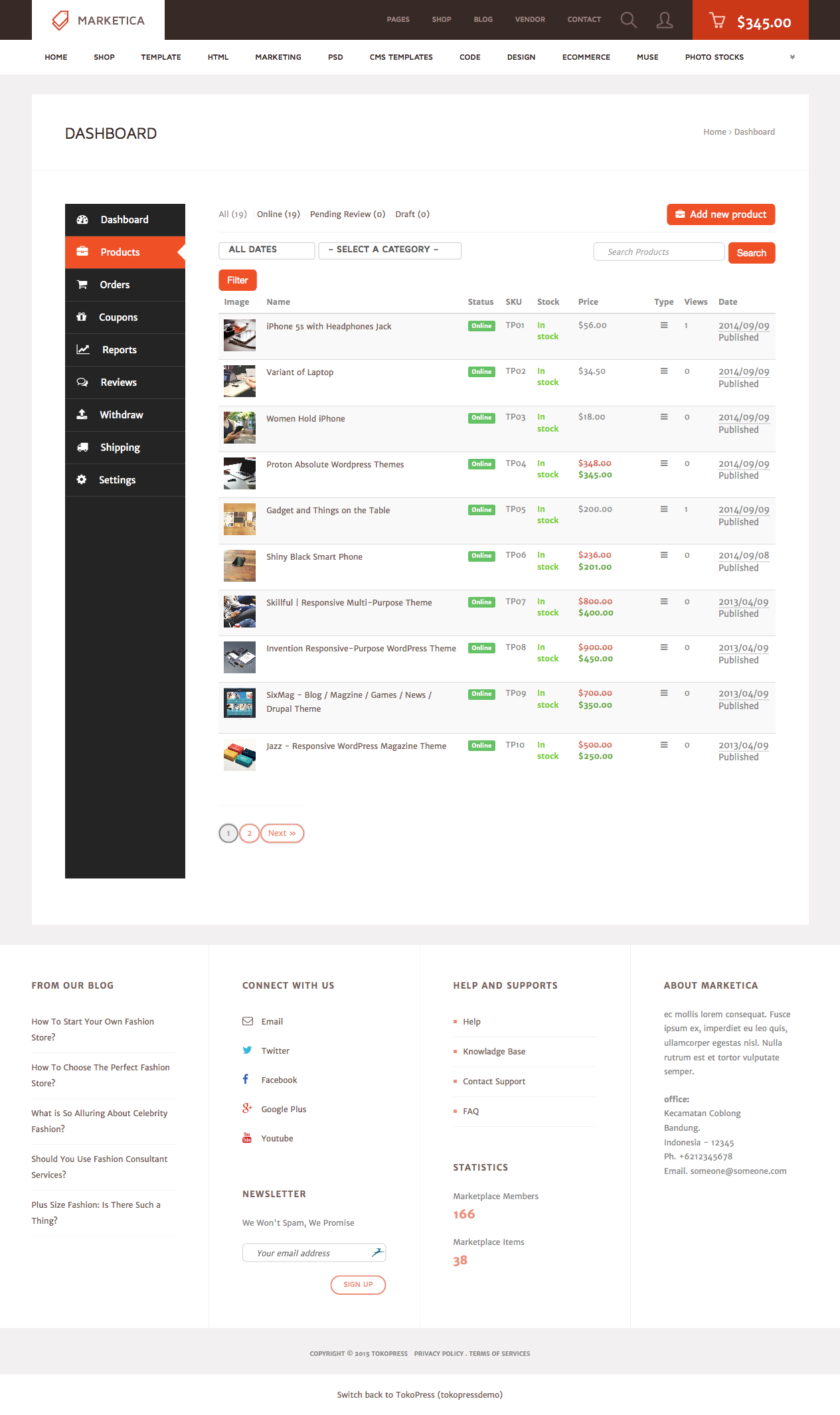
MARKETICA_PREVIEW/28_marketica2_dokan_vendor_dashboard_products_page.png
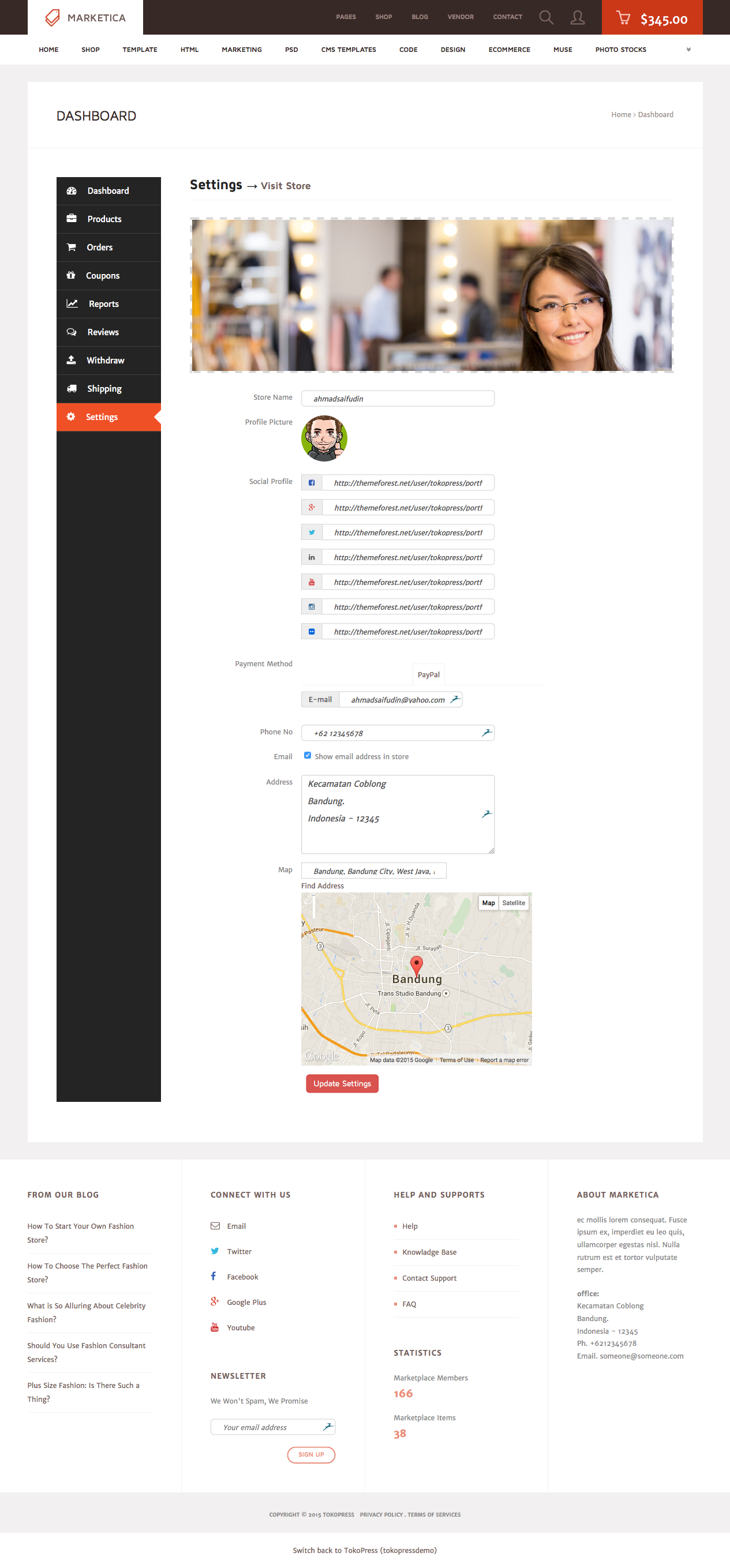
MARKETICA_PREVIEW/29_marketica2_dokan_vendor_dashboard_settings_page.png
 Promo
Promo
 Login
Login
 Daftar
 Whatsapp
 Live Chat